|
By Eric Lawrey, Copyright 1997-2001
An OFDM system was modelled using Matlab
to allow various parameters of the system to be varied and tested. The
aim of doing these simulations was to measure the performance of OFDM under
different channel conditions, and to allow for different OFDM configurations
to be tested. Four main criteria were used to assess the performance of
the OFDM system, which were its tolerance to multipath delay spread, peak
power clipping, channel noise and time synchronization errors.
2.1 OFDM Model Used
The OFDM system was modelled using Matlab
and is shown in Figure 16. A brief description of the model is provided
below.
Figure 16 OFDM Model used for simulations
2.1.1 Serial to Parallel Conversion
The input serial data stream is formatted
into the word size required for transmission, e.g. 2 bits/word for QPSK,
and shifted into a parallel format. The data is then transmitted in parallel
by assigning each data word to one carrier in the transmission.
2.1.2 Modulation of Data
The data to be transmitted on each carrier
is then differential encoded with previous symbols, then mapped into a
Phase Shift Keying (PSK) format. Since differential encoding requires an
initial phase reference an extra symbol is added at the start for this
purpose. The data on each symbol is then mapped to a phase angle based
on the modulation method. For example, for QPSK the phase angles used are
0, 90, 180, and 270 degrees. The use of phase shift keying produces a constant
amplitude signal and was chosen for its simplicity and to reduce problems
with amplitude fluctuations due to fading.
2.1.3 Inverse Fourier Transform
After the required spectrum is worked out,
an inverse fourier transform is used to find the corresponding time waveform.
The guard period is then added to the start of each symbol.
2.1.4 Guard Period
The guard period used was made up of two
sections. Half of the guard period time is a zero amplitude transmission.
The other half of the guard period is a cyclic extension of the symbol
to be transmitted. (As discussed in section 1.3.10). This was to allow
for symbol timing to be easily recovered by envelope detection. However
it was found that it was not required in any of the simulations as the
timing could be accurately determined position of the samples.
After the guard has been added, the symbols
are then converted back to a serial time waveform. This is then the base
band signal for the OFDM transmission.
2.1.5 Channel
A channel model is then applied to the
transmitted signal. The model allows for the signal to noise ratio, multipath,
and peak power clipping to be controlled. The signal to noise ratio is
set by adding a known amount of white noise to the transmitted signal.
Multipath delay spread then added by simulating the delay spread using
an FIR filter. The length of the FIR filter represents the maximum delay
spread, while the coefficient amplitude represents the reflected signal
magnitude.
2.1.6 Receiver
The receiver basically does the reverse
operation to the transmitter. The guard period is removed. The FFT of each
symbol is then taken to find the original transmitted spectrum. The phase
angle of each transmission carrier is then evaluated and converted back
to the data word by demodulating the received phase. The data words are
then combined back to the same word size as the original data.
2.1.7 OFDM simulation parameters
Table 9 shows the configuration used for
most of the simulations performed on the OFDM signal. An 800-carrier system
was used, as it would allow for up to 100 users if each were allocated
8 carriers. The aim was that each user has multiple carriers so that if
several carriers are lost due to frequency selective fading that the remaining
carriers will allow the lost data to be recovered using forward error correction.
For this reason any less then 8 carriers per user would make this method
unusable. Thus 400 carriers or less was considered too small. However more
carriers were not used due to the sensitivity of OFDM to frequency stability
errors. The greater the number of carriers a system uses, the greater it
required frequency stability.
For most of the simulations the signals
generated were not scaled to any particular sample rate, thus can be considered
to be frequency normalized. Three carrier modulation methods were tested
to compare their performances. This was to show a trade off between system
capacity and system robustness. DBPSK gives 1 bits/Hz spectral efficiency
and is the most durable method, however system capacity can be increased
using DQPSK (2 bits/Hz) and D16PSK (4 bits/Hz) but at the cost of a higher
BER. The modulation method used is shown as BPSK, QPSK, and 16PSK on all
of the simulation plots, because the differential encoding was considered
to be an integral part of any OFDM transmission.
(Addendum 10/2001:
Many OFDM systems now use coherent modulation instead of differential modulation
as coherent modulation allows the use of Quadrature Amplitude Modulation
(QAM) carrier modulation, which improves the spectral efficiency).
| Parameter |
Value |
| Carrier Modulation used |
DBPSK, DQPSK, D16PSK |
| FFT size |
2048 |
| Number of carrier used |
800 |
| Guard Time |
512 samples (25%) |
| Guard Period Type |
Half zero signal, half a cyclic extension of the symbol |
Table 9 OFDM system parameters used for the simulations
(Errata Note:
10/2001. The simulation results presented here show the overall Symbol
Error Rate (SER) rather than the Bit Error Rate (BER) as indicated on the
graph results and discussions. For BPSK the SER equals the BER, however
for QPSK the BER will be approximately half the SER. This is because two
bits of information are transferred for each QPSK symbol and typically
only single bit errors occur when suitable mapping is used (gray coding)
and the noise level is low. This approximation is valid for a SER below
approximately 1x10⁻². For 16PSK the same argument applies, thus the true
BER is approximately one quarter the SER).
2.2 OFDM Simulated Results
2.2.1 Multipath Delay Spread Immunity
For this simulation the OFDM signal was
tested with a multipath signal containing a single reflected echo. The
reflected signal was made 3 dB weaker then the direct signal as weaker
reflections then this did not cause measurable errors, especially for BPSK.
Figure 17 shows the simulation results.
It can be seen from Figure 17 that the
BER is very low for a delay spread of less then approximately 256 samples.
In a practical system (i.e. one with a 1.25 MHz bandwidth) this delay spread
would correspond to ~80 m sec.
This delay spread would be for a reflection with 24 km extra path length.
It is very unlikely that any reflection, which has travelled an extra 24
km, would only be attenuated by 3 dB as used in the simulation, thus these
results show extreme multipath conditions. The guard period used for the
simulations consisted of 256 samples of zero amplitude, and 256 samples
of a cyclic extension of the symbol. The results show that the tolerable
delay spread matches the time of the cyclic extension of the guard period.
It was verified that the tolerance is due to the cyclic extension not the
zeroed period with other simulations. These test however are not shown
to conserve space.
Figure 17 Delay Spread tolerance of ODFM
For a delay spread that is longer than
the effective guard period, the BER rises rapidly due to the inter-symbol
interference. The maximum BER that will occur is when the delay spread
is very long (greater then the symbol time) as this will result in strong
inter-symbol interference.
In a practical system the length of the
guard period can be chosen depending on the required multipath delay spread
immunity required.
2.2.2
Peak Power Clipping
It was found that the transmitted OFDM
signal could be heavily clipped with little effect on the received BER.
In fact, the signal could the clipped by up to 9 dB without a significant
increase in the BER. This means that the signal is highly resistant to
clipping distortions caused by the power amplifier used in transmitting
the signal. It also means that the signal can be purposely clipped by up
to 6 dB so that the peak to RMS ratio can be reduced allowing an increased
transmitted power
Figure
18 Effect of peak power clipping for OFDM
2.2.3 Gaussian Noise Tolerance of OFDM
It was found that the SNR performance of
OFDM is similar to a standard single carrier digital transmission. This
is to be expected, as the transmitted signal is similar to a standard Frequency
Division Multiplexing (FDM) system. Figure 1 shows the results from the
simulations. The results show that using QPSK the transmission can tolerate
a SNR of >10-12 dB. The bit error rate BER gets rapidly worse as the SNR
drops below 6 dB. However, using BPSK allows the BER to be improved in
a noisy channel, at the expense of transmission data capacity. Using BPSK
the OFDM transmission can tolerate a SNR of >6-8 dB. In a low noise link,
using 16PSK can increase the capacity. If the SNR is >25 dB 16PSK can be
used, doubling the data capacity compared with QPSK
Figure
19 BER verse SNR for OFDM using BSPK, QPSK and 16PSK
(Errata 10/2001:
The simulation results shown in Figure 19 are slightly incorrect due to
the calculation of the noise level in the simulation. The simulations shown
above calculated the signal to noise ratio based on the power of the time
domain signal waveform and the power of the time domain noise waveform,
with no consideration of the signal bandwidth. At the receiver the signal
is filtered by the FFT stage, thus making the receiver only see noise within
the signal bandwidth. The simulations were performed using 800 carriers
and generated using a 2048-point IFFT. The nyquist bandwidth is half the
transmission sample rate as the signal is real (i.e. no imaginary components)
and so the nyquist bandwidth corresponds to 1024 carriers. The signal bandwidth
is thus 800/1024 = 0.781 or 78.1% of the nyquist bandwidth. Since the receiver
was only seeing 78.1% of the total noise the error rate is lower than it
should be. The correct SNR values can be found by adding 1.07 dB (10.log10(0.781))
to the scale in Figure 19. Also note the simulation results actually show
the Symbol Error Rate rather than the Bit Error Rate).
2.2.4 Timing Requirements
One of the big questions at the start of
the thesis was how tolerant OFDM would be to a starting time error. The
problem was that when an OFDM receiver is initially switched on it will
not be synchronized with the transmitted signal. So a synchronization method
was required. The proposed method was that the OFDM signal could be broken
up into frames, where each frame transmits a number of symbols (somewhere
between 10-1000). At the start of each frame a null symbol is transmitted,
thus allowing the start of the frame to be detected using envelope detection.
However using envelope detection only allows the start to be detected to
within a couple of sample, depending on the noise in the system. It was
not known whether this timing accuracy was sufficient. This method was
used for the synchronization in the practical tests performed. (See section
2.3)
Figure 20 shows the effect of start time
error on the received BER. This shows that the starting time can have an
error of up to 256 samples before there is any effect of the BER. This
length matches the cyclic extension period of the guard interval, and is
due to the guard period maintaining the orthogonality of the signal
In any practical system, the timing error
made be either early or late, thus any receiver would aim for the middle
of the expected starting time to allow for an error of ±128 samples.
In addition, if the signal is subject to any multipath delay spread, this
will reduce the effective stable time of the guard period, thus reducing
the starting time error tolerance
Figure
20 Effect of frame synchronization error on the received OFDM signal.
2.3
Practical Measurements
A set of practical measurements was made
on the OFDM system. This was done so that the simulated results could be
partly verified and so that difficulties in implementing a practical system
could be tackled, and to measure some effects which were hard to simulate.
The practical measurements were performed
using a Personal Computer (PC) as an OFDM generator and receiver. A Matlab
program was developed to process the input and output signals and a Sound
Blaster 16 card was used to play the transmitted OFDM signal, and used
to record the received signal. Only one PC was available with a sound card
and so the transmission was performed in two steps. The transmitted signal
was generated using Matlab then played out the sound card and recorded
onto an audio recorder. This signal was then played back and re-recorded
by the sound card on the computer. The received signal was then processed
using a Matlab script. Two different audio recorders were tested, as each
gave a different performance.
The first used was the HiFi stereo audio
track on a high quality VCR (Panasonic Super-VHS FS90). This gave a high
quality audio channel (SNR >90dB, 20Hz - 20kHz range, and crystal accuracy
stability of frequency (0.005%)), which was a good model for a near perfect
radio channel
The system was also tested using an audio
tape player. The tape player had a much poorer performance, in noise (~50dB
SNR), audio bandwidth (20Hz-15kHz), and particularly frequency stability
(2%). This provided a good test of the performance of OFDM in a channel
with very poor frequency stability
2.3.1
Extended Model
The basic OFDM model used for the simulations
(see section 2.1) was extended to allow for the received signal to be automatically
be synchronized to the OFDM frame structure, and for large data files to
be able to be transmitted.
2.3.2
Transmission Protocol
A basic frame structure was used to allow
the receiver to synchronize with the transmitted signal. The frames were
marked out by having a null symbol (zero amplitude) between frames (see
Figure 21), allowing the start of each frame to be detected using an envelope
detector in software. The transmitted signal consisted of a number of frames
(typically 1- 100), with a preamble at the start and a post signal at the
end (see Figure 22). The preamble was used to provide the start time of
the first frame and consisted on a mixture of tones. This was required
so that the envelope detector had a signal to initialise the filtering
required.
Figure
21 Frame Structure, showing the null symbol between frames
The envelope detector was implemented by
rectifying the input signal then applying a moving average filter to the
signal. The length of the filter was made exactly the same length as the
null symbol. This results in the filtered signal having a minimum amplitude
at the start of a frame. This minimum was used to find the starting location
in which to decode the entire frame. Each frame consists of a number of
symbols (typically 5-40) that contain the actual data

Figure
22 Frame Structure used for the OFDM transmission
2.3.3
Video Recorder
The first simulated channel used was the
audio track of a VCR
2.3.3.1
Number of Carriers Used
For an OFDM system, the number of carriers
used in the transmission determines several parameters about the system.
These include the processing speed required, the symbol time (thus the
maximum delay spread that can be tolerated), the number of users the available
bandwidth can be split over (i.e. one carrier per user), and the frequency
stability required.
Since there was no easy way of simulating
this effect with the Matlab model developed, it was decided to measure
it in a practical way. This was done by varying the number of carriers
used when transmitting the OFDM over the link simulated by the VCR. The
frequency stability of the VCR’s recording and playing was considered to
be approximately the same for each of the tests performed. This allowed
the relative effect of varying the number of carriers for a fixed frequency
stability.
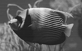
The data used in the transmission was that
of a grey-scale bit-map image of a fish. The original of the image is show
below in Figure 23

Figure
23 Image used in transmission tests
The transmission was sent using 256PSK.
This was chosen because it gave the highest transmission efficiency (~8
bits/Hz), thus resulting in the smallest transmission data size. By sending
each 8-bit grey scale pixels as one carrier per symbols, any phase errors
in the transmission directly correspond to a change in the intensity of
the received signal. This allows the phase angle errors to be judged from
the image quality. Since the phase error due to a frequency offset or phase
noise has the same effect on the received data as gaussian noise, it can
be effectively converted to an equivalent signal to noise ratio of the
received image.
The image quality and phase error was measured
at different number of carriers used to transmit the signal.
Figure
24 Performance of the OFDM using the VCR as a channel, as a function of
the number of carriers used
Figure 24 show the effect that increasing
the number of carriers had on the received signal. It can be seen that
the larger the FFT size (and number of carriers used), the worse the performance
of the system. This is due to the VCR having a fixed frequency stability
thus the closer the carriers are in the transmission, the worse the effect
of the frequency error. The SNR of the received image for an FFT size of
2048 was only 20 dB. This is much worse then the SNR ratio that would be
expected from the channel noise. The VCR has excellent noise performance
(>70-90 dB SNR for gaussian noise) however this limit is no where near
reached due to frequency stability problems causing an effective SNR of
between 10-3 0dB. This indicates that the performance of the system is
not limited by the gaussian noise of the system, but the frequency stability
Since the frequency stability of the is
such a problem in an practical radio OFDM system the receiver would have
to be frequency locked to the transmitter in order achieve the maximum
performance
| Received Image from VCR audio channel |
Error in received image (contrast enhanced to show the errors) |
16384 point FFT, 5600 carriers |
16384 point FFT, 5600 carriers |

256 point FFT, 75 carriers |
256 point FFT, 75 carriers |
Table
10 Received OFDM images using the audio channel of a VCR
Table 10 shows some of the received images
that were used to generate Figure 24. It can be seen that the image transmitted
using 5600 carriers has bands in the image, due to the phase errors (and
thus pixel intensity errors) in the transmission. Also some of the pixels
that are white (on the top of the fish) have wrapped round to show white.
This is due to the received phase error causing a wrap around from 255
to 0 in intensity
2.3.4
Peak OFDM Performance for the VCR link
After trying out different OFDM system
parameters such as the number of carriers used, system bandwidth and guard
period length, it was found that very high spectral efficiency could be
achieved. Figure 25 shows the maximum performance that could be achieved
on the VCR audio track.
Figure
25 Image transferred at 134kbps in an 18.2kHz bandwidth on the VCR audio
channel, using 210 carriers.
The image of the fish was transferred using
256PSK. The total transmission time was 4.54 seconds for 76246 bytes of
data, with only 18.2 kHz bandwidth. This gives a spectral efficiency of
7.4 bits/Hz. This is just under the theoretical limit of 8 bits/Hz for
256PSK and is due to overhead in the guard period and frame symbols. The
signal was generated using a 512-point FFT, using 210 carriers, and a guard
period of 32 samples. The carriers used were based on the frequency response
of the VCR link measured in section 2.3.4.2, so that the maximum bandwidth
could be used
The received image in Figure 25 has slight
phase errors, which are just noticeable as bands in the image. Also some
pixel on the top fin of the fish have wrapped around from white to black.
2.3.4.1 Peak Power Clipping
The clipping tolerance of the OFDM signal
was tested to verify that OFDM can handle a large amount of peak power
clipping before any significant increase in the bit error rate (BER) occurs.
The simulations indicated that OFDM could handle up to 9 dB of clipping
(for QPSK) before the BER became detectable. This result was slightly surprising
as any non-linearity in the system lead to intermodulation distortion.
Thus the initial expectation was that OFDM would be susceptible to any
clipping of the signal
The clipping of the signal was performed
during the recording from the VCR back to the computer for decoding. The
clipping of the signal was achieved by using back- to-back germanium diodes
across at the output of the VCR with a resistor in series with the VCR
to limit the current flow. The signal was observed on a CRO and increased
in amplitude until clipping occurred. The peak power clipping was measured
by finding the ratio of the peak signal level before clipping, to the peak
signal level after clipping
| Peak Signal before clipping (Vp-p) |
Peak Signal after clipping (Vp-p) |
Calculated Peak Power Clipping (dB) |
Measured BER of received signal |
Predicted BER from simulation |
| 1.45 |
0.72 |
6.08 |
<0.00006 |
|
| 1.88 |
0.80 |
7.45 |
<0.00006 |
|
| 2.01 |
0.805 |
7.95 |
<0.00006 |
|
| 2.65 |
0.853 |
9.85 |
0.0004 |
<0.00009 |
| 3.55 |
0.917 |
11.8 |
0.0036 |
0.0038 |
| 4.6 |
0.935 |
13.84 |
0.0125 |
0.0208 |
Table 11 Results of clipping the OFDM signal, showing the resulting BER
Table 11 shows the measured error rates
when the signal was clipped, and the expected BER based on the simulations.
The BER was found to be too small (<0.00006) for peak power clipping
up to 8 dB. The BER was only detectable for peak power clipping of >8-10
dB, matching the expected result of 9 dB measured from the simulations
(see section 2.2.2). For high levels of clipping, from 12- 14 dB, the measured
BER was actually lower then the simulated results. This is probably due
to the fact that the germanian diodes used for clipping of the signal were
not clipping as abruptly as in the simulation resulting in lower intermodulation
distortion and a lower BER.
2.3.4.2 VCR performance
The audio performance of the VCR link was
measured so that the quality of the channel used for the practical measurements
could be assessed. The loop back frequency response of the channel was
measured by using the sound card to generate white noise. This noise was
then recorded on the VCR, then played back and recorded back on to the
computer. The power spectral density of the noise was then measured giving
an estimate frequency response of the system. Since the signal was generated
from the sound card the measured frequency response is the combined performance
of the Sound Blaster 16 card and the VCR.
Figure 26 shows the frequency response
of the VCR link used.
The frequency stability of the VCR is quoted
by the manufacturer as 0.005%. This was verified by recording a 10 kHz
sine wave on to the VCR using the sound card to generate the signal. The
frequency of the played back signal was measured using a frequency meter.
It was found that the played back signal to be stable to better then the
resolution of the frequency meter used (i.e. 10.000 kHz). Thus the sound
card, VCR combination was stable to better then 0.01%
Figure 26 Record / Play back frequency response of the Panasonic FS90 VCR / Sound
Blaster 16 combination using a sample rate of 44.1kHz
2.3.5 Audio Tape Player
After much success in using the VCR as
a link, the OFDM system was also tested using an audio tape player as the
channel. The audio tape player used is not frequency locked, as with the
VCR, thus has a very poor frequency stability. This can lead to a large
frequency offset error in the recording. Since OFDM is very susceptible
to frequency offset errors, the performance of the system was poor on the
tape player
2.3.5.1 Carrier Number
Several test OFDM transmissions were tried
using the tape player as a channel. It was found that the only way to successfully
store an image on the tape player was to greatly reduce the number of carriers
used. Table 12 shows two images that were recorded on the audiotape play
then recorded and decoded back onto the computer. It can be seen that the
image quality when using only 5 carriers was much better than using 21
carriers. The image transmitted using 21 carriers, has lines and smears
through it due to phase errors. This is due to the frequency instability
of the tape player.
| Received Image |
Spectrum of the received signal |
64 point FFT, 21 carriers |

(Click the image for a larger version)
|

16 point FFT, 5 carriers
|
(Click the image for a larger version)
|
Table 12 Received images from the audio tape player, using OFDM with 5 and 21
carriers.
2.3.5.2 Tape Player Performance
The frequency stability and frequency response
of the tape player were measured to assess the effective quality of the
channel. All tests were performed using the audio tape player in conjunction
with the Sound Blaster 16 card, thus the measurements are the combination
of their performances
The measurements were performed using the
same technique used for performance measurement of the VCR (see section
2.3.4.2).
Frequency Stability
A 10 kHz tone was generated using the sound
card by playing a windows 3.1 WAV file generated by a Matlab script. This
tone was then recorded on the tape player. The frequency and amplitude
of the played back signal was then measured over a 10 second period. This
time length was used because it was approximately the same length of time
that is taken in transmitting the fish image. The results are shown below
in Table 13
| |
Frequency (kHz) |
Amplitude Variation (dB) |
| Max |
10.000 |
0.21 |
| Mean |
9.987 |
0.01 |
| Min |
9.823 |
-0.25 |
Table 13 Frequency and amplitude fluctuations in a 10second, 10kHz tone played
back from the audio tape player
Thus the frequency offset is -0.13% and
the variation is 1.77%. The level of frequency instability is very high
as even for only 21 carriers this represents the carrier frequencies shifting
by up to 40% of a carrier spacing. This frequency instability would cause
large phase errors to occur
Frequency Response
The tape player / Sound Blaster 16 frequency
response is shown below in Figure 27. The bandwidth of the tape player
is about 15 kHz, plus the response is reasonably flat (± 3 dB).
The frequency response of the tape player should not cause any significant
problems for the OFDM signal
Figure
27 Record / Play back frequency response of the JVC TD-W444 / Sound Blaster
16 with a sample rate of 44.1kHz
2.4
Picture quality verse signal to noise ratio
This section describes some work that was
done relating to improving the degradation performance of OFDM when the
channel noise becomes very high. One problem with many digital communication
systems is that the performance of the system is fine, up to some critical
channel noise level, above which the system fails very quickly. This can
cause potential problems for wireless telecommunications where the received
signal quality can vary greatly depending of the location of the mobile
station. This problem leads to drop outs in the signal, decreasing the
reliability of the system. It would be far better if the system simply
gave a worse voice or image quality under high noise conditions, rather
then completely loosing the signal
It was noticed when doing the practical
measurements on OFDM (see section 2.3) that the received quality of the
image was very good using 256PSK even though the measured error rate was
very high. Using 256PSK to transmit the image is similar to sending an
analog transmission as channel noise simply appears as noise in the image.
The main question was, does sending the image using 256PSK result in better
performance then QPSK in a high noise environment? To answer this question,
a simple comparison was set up
2.4.1 Setup
The same Matlab scripts were used for this
test as in the previous practical measurements, however the signal wasn’t
recorded to any external audio channel as in the practical tests. The channel
noise was simulated using the same model as used in the OFDM simulations
(see section 2.1). The signal to noise ratio (SNR) of the channel was varied
from 0 dB up to 15 dB, with the image quality measured at 3 dB increments.
No forward error correction was used for either modulation technique
Using 256PSK allows 8 bits to be sent on
each carrier per symbol, compared to only 2 bits for QPSK. Thus, 256PSK
on its own allows for up to 4 times the transmission data rate. Since the
aim of the experiment was to compare the relative performance differences
between QPSK and 256PSK under the same transmission bandwidth and data
rate, the 256PSK transmission was slowed down by 4 times to have the same
transmission rate. This was achieved by repeating the 256PSK symbols four
times, thus reducing the data rate to the same as using QPSK. The four
repetitions were then combined at the receiver by averaging the received
demodulated phase angle. This averaging reduces the received phase noise
by up to 6 dB.
Transmitting the signal using 256PSK with
linear mapping of the pixel intensity is very similar to transmitting the
imaging in an analog manner. This modulation technique is essentially linear
Phase Modulation. Transmitting the signal in an analog manner result in
a direct mapping between phase errors caused by the channel, and amplitude
noise (pixel intensity) in the received image. Using a linear mapping tends
to reduce the chance of the large catastrophic errors that can occur when
sending digital data that is not mapped in a linear manner.
However when transmitting using a standard
digital modulation technique such as QPSK, the SNR of the demodulated image
can be much higher then the channel SNR, provided the channel SNR is greater
then ~10 dB. This is because small phase errors are not big enough to cause
a bit error and thus no noise is seen on the received signal. However when
the SNR of the channel becomes worse (< 10 dB), phase errors cause the
received signal to be misread thus causing bit errors. Since the mapping
of the bits to the amplitude of the transmitted signal are not linearly
related, a single bit error can cause a significant error in received amplitude.
This results in a rapid drop in performance of the received signal as the
SNR of the channel drops below ~10 dB for QPSK.
2.4.2 Results
Figure 28 shows how the signal to noise
of the received image decreases as the signal to noise ratio of the transmission
channel also worsens. It can be seen that the 256PSK signal performs better
then the QPSK transmission below a channel SNR of 9 dB.
Figure 28 Comparison between the received image SNR using QPSK and 256PSK verses
the SNR.
For a channel SNR of 0 - 6 dB the 256PSK
signal averaged approximately 7 - 9 dB better picture quality then the
QPSK signal. This gain is to be expected as there are two reasons for the
improvement. Firstly, the signal has been averaged (thus reducing the phase
noise), and that the phase angle mapping used for 256PSK, as the 256PSK
signal is averaged over 4 repeats, giving approximately a 6 dB improvement
compared with the channel SNR.
Table 14 shows some of the received images.
It is easy to see that the image quality of the signal transmitted using
256PSK is much better then using QPSK
| QPSK |
256 PSK with 4 times data averaging |
 SNR = 12dB SNR = 12dB |
 SNR = 12dB SNR = 12dB |
 SNR = 6dB SNR = 6dB |
 SNR = 6dB SNR = 6dB |
 SNR = 0dB SNR = 0dB |
 SNR = 0dB SNR = 0dB |
Table 14 Comparison between QPSK and 256PSK for transmitting an image under noisy
conditions.
It was found that the picture sent using
QPSK had a much better quality then the 256PSK signal in a low noise channel,
where as the 256PSK performed better then QPSK under high noise conditions
with a SNR < 9 dB.
Note: the performance of the QPSK signal
can be significantly improved using advanced forward error correction techniques.
This however cannot be applied to 256PSK using these same techniques as
the matching between the phase mapping and the pixel intensity will be
lost and the error is too high (typically 0.8-0.95 for SNR <12 dB) for
most error correction to work successfully. The use of forward error correction
techniques may result in the performance of QPSK and 256PSK being the same
or QPSK performing better
2.5 Mathematical Model for OFDM performance
The aim was to develop a mathematical model
of the performance (BER) of OFDM verses the channel noise. This was so
that the simulated results could be verified, and to get a more in depth
understanding of the transmission mechanism.
The model developed is based on the transmission
modulation technique being phase shift keying, and that the channel noise
is gaussian noise (i.e. white noise)
2.5.1 RMS Demodulated Phase Error
If we assume that the transmission modulation
method used is phase shift keyed then any noise added to the transmitted
signal will result in a phase error. If we look at the IQ diagram of the
transmitted signal then the transmitted signal will be a phasor of fixed
magnitude, and of phase corresponding to the data to be transmitted. The
noise can then be considered as the random vector added to the transmitted
signal. The magnitude of the phase error depends on two things, the relative
phase angle of the noise vector, and the magnitude of the noise vector
The received vector will be the vector sum
of the transmitted signal and the noise. If we assume that the noise is
a constant magnitude vector equal to its RMS magnitude, and that it has
a random phase angle then the problem of working out the received angle
would be as follows
2.5.2 BER verses Channel Noise
Figure 29 show the effect of noise on the
received phase angle. If we let the amplitude of the transmitted signal
be 1, and the length of the noise vector be A with angle f, then the received
phase error is θerr.
Figure 29 Received Phasor, showing effect of noise on the received phase angle.
Using trigonometry,


Since,
Therefore,
The signal to ratio determines the relative
amplitude of the received signal and the noise level. Since the signal
is scaled to an amplitude of 1, the amplitude of the noise is:

Note: The SNR is base on the amplitudes
of the signals thus must be scaled correctly when converting it to dB
If we substitute this in we get,
The noise signal can be of any phase angle.
What we need is to find is the RMS phase error, so if we find the average
phase error (assuming the noise phase angle is always positive) then this
can be scaled to find the RMS error. The average phase angle can be found
by integrating θerrover
a half circle, i.e j varies
from 0 to p
The RMS phase error will be greater by root 2, thus
Equation 1
This equation was was used to predict the
RMS phase error for different channel SNRs. This was compared with the
results obtained using the simulation of OFDM. Figure 30 shows that the
predicted results based on the above mathematical derivation match the
simulated results very well
Figure 30 Comparison between the measured RMS phase error using the simulations
and the predicted result. (Also shown in Table 22)
Once the RMS phase error has been calculated
the BER can be easily calculated using simple statistics. The RMS phase
error is the standard deviation of the phase error. An error will occur
if the phase error gets bigger then the maximum allowed for the modulation
method used. Thus the BER can be determined by finding the probability
of the phase error being greater the plus, minus the maximum phase error
for a standard deviation equal to the RMS phase error. This is outlined
in the following example
The Bit Error Rate (BER) of an OFDM link
can be predicted based on the channel signal to noise ratio (SNR) and phase
modulation used (e.g. BPSK, QPSK, etc). This is done by finding out what
the expected RMS phase error (θerror(rms))
there will be on the signal (due to the channel noise). The bit error rate can
then be found by comparing the magnitude of the RMS phase error to that
of the maximum phase allowed for the particular phase modulation used
(θmax).
2.5.3 Maximum Allowable Phase Angle
θmax is
the maximum phase error allowed on the received symbol, before an error
will occur on the received word
Figure 31 IQ diagram for QPSK, showing the phase locations for data (crosses)
and that θmax
is 45 degrees
| Modulation Technique |
Maximum Phase Error Allowed θmax in degrees |
| BPSK |
90 |
| QPSK |
45 |
| 16PSK |
11.25 |
| 256PSK |
0.70313 |
Once θmax and θerror(rms)
have been established, Z can be calculated, and the BER found from Table
22

Example
For a QPSK transmission if the signal
to noise ratio (SNR) of the channel is 10dB, find the BER:
Note: Table 21 shows a summary calculated
from Equation 1
From Table 21, θerror(rms)=16.5 degrees,
For QPSK,θmax=45 degrees,
Therefore,
From Table 22 the BER is between 0.0053
and 0.0091, with a result of 0.0077 if the results are interpolated
2.6 OFDM system implementation
The proposed final application for OFDM
is to use it for wireless communications systems such as cellular mobile
phone systems, fixed wireless phone systems, wireless data links and wireless
computer local area networks. If OFDM is to be used in any of these applications
then the bandwidth used must be sufficiently high to compete with other
radio technologies. This section discusses the processing power required
to implement a practical OFDM system
An OFDM system mainly involves digital
signal processing, thus the main focus of the performance of the system
depends on the availability of high performance signal processing. There
are two main ways in which the OFDM signal can be processed, which are
using a general purpose DSP, or by implementing the processing in hardware
using customized IC’s.
2.6.1 Using general purpose DSPs
There are several processing stages required
to generate and receive an OFDM signal. However most of the processing
is required in performing the Fast Fourier Transform (FFT).
The complexity of performing an FFT is
dependent on the size of the FFT. The larger the FFT the greater the number
of calculations required, however since as the symbol period is longer
the increased processing required is less then the straight increase in
processing to perform a single FFT. Table 15 shows the number of calculations
required for an FFT (radix-2) of size N, and also the relative processing
for various FFT sizes. It can be seen that because the symbol period increases
with a larger FFT that the extra processing required is minimal
| Size FFT (N) |
Total number of complex calculations (values from [21]) |
Relative processing required for OFDM generation (normalized to 1024 point FFT) |
| 32 |
240 |
0.5 |
| 64 |
576 |
0.6 |
| 128 |
1344 |
0.7 |
| 256 |
3072 |
0.8 |
| 512 |
6912 |
0.9 |
| 1024 |
15360 |
1.0 |
| 2048 |
33792 |
1.1 |
| 4096 |
73728 |
1.2 |
Table 15 Processing complexity for FFT
The processing efficiency of a DSP processor
depends on the architecture of the processor, however for most single instruction
DSP’s the number of cycles required to calculate an FFT is twice the total
number of calculations shown in Table 15. This is due to complex calculations
requiring two operations per calculation
Required Processing Power
To get an estimate of the processing power
required to implement a practical phone system, lets consider an example
| Basic System Parameter |
Value |
| Total Bandwidth |
1.25MHz |
| User Capacity |
64 users |
| Modulation Used |
QPSK |
| FFT size |
2048 |
| Guard period |
512 samples |
Table 16 Example OFDM system
Table 16 shows a example system. From these
basic system parameters the required number of carriers, user data rate
and symbol rate can be calculated. These are shown in
| Derived System Parameter |
Value |
| No. of active carriers |
832 |
| Data Rate of each User |
39 kbps |
| Useful symbol time |
666 msec |
| Total symbol time |
833 msec |
Table 17 Derived system parameters for the example OFDM system
From Table 15 the number of complex calculations
required for a 2048 point FFT is 33792. The maximum time that can be taken
in performing the calculation is once every symbol thus once every 833 msec.
If we assume that the processor used requires 2 instructions to perform
a single complex calculation, and that there is an overhead of 30% for
scheduling of tasks and other processing. The minimum processing power
required for this is then:
Thus the transmitter requires >105MIPS
in order to implement to OFDM transmitter. The receiver will require just
as much as the transmitter, thus a full OFDM transceiver will require >210MIPS.
This is a lot of processing required. Most current cheap DSPs are only
25-50MIPS (i.e. AD2181 is 33MIPS). Currently the fastest general purpose
DSP is produced by Texas Instruments. The TMS320C62xx is capable of up
to 1600MIPS which would make it plently fast enough for an OFDM transceiver.
However, the price of the TSM320C62xx is not known and is expected to be
very expensive
(Addendum 10/2001:
Texas Instruments are now producing the TMS320C64xx, which is the next
generation of fixed point DSP’s. These processors are capable of up to
4800 MIPS).
OFDM clearly requires a large amount of
porcessing power, however since computer technology is advancing so fast
this may not become a problem in the future
2.6.2 Future DSP Processing Power
Computer technology, and signal processing
technology is improving at a rapid rate. The IC industry is on a self-prescribed
course of development of ever-smaller devices and faster circuits. By the
year 2000, logic IC will employ up to 60 million transistors and operate
at speeds of over 1GHz.
Figure 32 shows the expected performance
increase in general purpose microprocessors until the year 2010. If this
is considered as an indicator for DSP improvement in speed, this shows
that for the next 5 years we can expect a speed improvement in processing
of greater than 5 times. Thus an OFDM system will be easily achievable
using general purpose DSPs in 5 years time
(Addendum 10/2001:
Texas Instruments announced during 1999 that they predict that by 2010,
Digital Signal Processors will be capable of more than 1 Trillion Operations
Per Second, www.ti.com/sc/docs/news/1999/99086.htm)
Figure 32 The performance of general-purpose microprocessors will climb from 100
million operations per second in 1995 to more than 10 billion by 2010 (Source
[20])
2.6.3 Hardware FFT Implementation
Another way of implementing the FFT processing
required for generating and receiving the OFDM signal is by doing the FFTs
in hardware using FFT IC’s. Several 1024 point FFT chips are shown in Table
18. For the previos example a 2048 point FFT needed to be performed in
less then 830 msec.
This is much greater then the execution time required by any of the FFT
Ics in Table 18. Although these Ics only perform a 1024point FFT, clearly
the processing can be easily achieved using hardware implementation of
the FFT processing
| Processor |
Year |
Datapath Width (bits) |
Execution Time (1024-pt FFT) |
Number of Chips Required |
Pins |
Power (mW) |
| Cobra (Colorada State) |
1994 |
23 |
9.5 msec |
>16 |
391 |
7700 |
| PDSP16510A (Plessey) |
1989 |
16 |
98 msec |
1 |
84 |
3000 |
| DSP-24 (DSP Architectures) |
1997 |
24 |
21 msec |
7 |
308 |
3500+ |
| Spiffe ULP (Stanford) |
1995 |
20 |
61 msec |
1 |
70 |
8 |
Table 18 1024 point FFT Chip Comparison
Next Chapter 3
|